#==========
Julia の修行をするときに,いろいろなプログラムを書き換えるのは有効な方法だ。
以下のプログラムを Julia に翻訳してみる。


正準判別分析
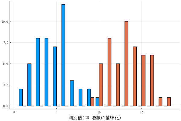
http://aoki2.si.gunma-u.ac.jp/R/candis.html ファイル名: candis.jl 関数名: candis 翻訳するときに書いたメモ 後の利用のために,結果を Dict で返すようにしているが,Dict が長すぎるか?? ==========# using Statistics, StatsBase, Rmath, LinearAlgebra, NamedArrays, Plots, StatsPlots function candis(data, group) vnames = names(data); data = Matrix(data); n, p = size(data) gname, ni = table(group) k = length(ni) grandmeans = vec(mean(data, dims=1)); groupmeans = zeros(p, k); groupvars = zeros(p, k); w = zeros(p, p); for (i, g) in enumerate(gname) data2 = data[group .== g, :] groupmeans[:, i] = mean(data2, dims=1) groupvars[:, i] = var(data2, dims=1) w .+= cov(data2, corrected=false) * ni[i] end means = hcat(grandmeans, groupmeans); b = (cov(data, corrected=false) .* n) .- w df1, df2 = k - 1, n - k Fvalue = [onewaytest(ni, groupmeans[i, :], groupvars[i, :]) for i = 1:p] pvalue = pf.(Fvalue, df1, df2, false) wilksFromF = df2 ./ (Fvalue .* df1 .+ df2) ss = cov(data, corrected=false) .* n .- w withincov = w ./ (n - k) sd = sqrt.(diag(withincov)) withinr = withincov ./ (sd * sd') eigenvalues, eigenvectors = eigen(b, w, sortby=x-> -x) nax = sum(eigenvalues .> 1e-10) axnames = "axis " .* string.(1:nax) eigenvalues = eigenvalues[1:nax] eigenvectors = eigenvectors[:, 1:nax] Λ = reverse(cumprod(1 ./ (1 .+ reverse(eigenvalues)))) chisq = ( (p + k) / 2 - n + 1) .* log.(Λ) lL = (1:nax) .- 1 df = (p .- lL) .* (k .- lL .- 1) pwilks = pchisq.(chisq, df, false) canonicalcorrcoef = sqrt.(eigenvalues ./ (1 .+ eigenvalues)) temp = diag(transpose(eigenvectors) * w * eigenvectors) temp = 1 ./ sqrt.(temp ./ (n - k)) coeff = eigenvectors .* temp' const0 = - grandmeans' * coeff coefficient = cat(coeff, const0, dims=1) stdcoefficient = coeff .* sqrt.(diag(withincov)); centroids = groupmeans' * coeff .+ const0; canscore = data * coeff .+ const0; structure = zeros(p, nax); for i = 1:nax data2 = hcat(canscore[:, i], data); ss = zeros(p + 1, p + 1) for j = 1:k dss = data2[group .== gname[j], :] ss .+= cov(dss, corrected=false) * ni[j] structure[:, i] = (ss[:, 1] ./ sqrt.(ss[1, 1] .* diag(ss)))[2:end] end end d = zeros(n, k); for i = 1:n for j = 1:k d[i, j] = sum( (canscore[i, :] .- centroids[j, :]) .^ 2) end end pvalue2 = pchisq.(d, p, false) pBayes = exp.(-d ./ 2) .* ni'; pBayes = pBayes ./ sum(pBayes, dims=2) classification = [gname[argmax(pBayes[i, :])] for i = 1:n] real, pred, correcttable = table(group, classification) correctratio = 100sum(diag(correcttable)) / n obj = Dict(:means => means, :b => b, :w => w, :withincov => withincov, :withinr => withinr, :eigenvalues => eigenvalues, :wilksFromF => wilksFromF, :Fvalue => Fvalue, :df1 => df1, :df2 => df2, :pvalue => pvalue, :Λ => Λ, :chisq => chisq, :df => df, :pwilks => pwilks, :canonicalcorrcoef => canonicalcorrcoef, :stdcoefficient => stdcoefficient, :structure => structure, :coefficient => coefficient, :centroids => centroids, :canscore => canscore, :pBayes => pBayes, :pvalue2 => pvalue2, :classification => :classification, :correcttable => correcttable, :real => real, :pred => pred, :correctratio => correctratio, :group => group, :ngroup => k, :nax => nax, :vnames => vnames, :gname => gname, :axnames => axnames) end function table(x) # indices が少ないとき indices = sort(unique(x)) counts = zeros(Int, length(indices)) for i in indexin(x, indices) counts[i] += 1 end return indices, counts end function table(x, y) # 二次元 indicesx = sort(unique(x)) indicesy = sort(unique(y)) counts = zeros(Int, length(indicesx), length(indicesy)) for (i, j) in zip(indexin(x, indicesx), indexin(y, indicesy)) counts[i, j] += 1 end return indicesx, indicesy, counts end function onewaytest(ni, mi, vi) n = sum(ni) k = length(ni) gm = sum(ni .* mi) / n df1, df2 = k - 1, n - k return (sum(ni .* (mi .- gm).^2) / df1) / (sum( (ni .- 1) .* vi) / df2) end function printcandis(obj) vnames = obj[:vnames] gname = obj[:gname] axnames = obj[:axnames] p = length(vnames) n = size(obj[:canscore], 1) println("\n全体および各群の平均値\n", NamedArray(obj[:means], (vnames, vcat("grand mean", gname)))) println("\n群間平方和\n", NamedArray(obj[:b], (vnames, vnames))) println("\n群内平方和\n", NamedArray(obj[:w], (vnames, vnames))) println("\n平均値の差の検定(一変量;一元配置分散分析)\n", NamedArray(hcat(obj[:wilksFromF], obj[:Fvalue], repeat([obj[:df1]], p), repeat([obj[:df2]], p), obj[:pvalue]), (vnames, ["Wilks", "F value", "df1", "df2", "p value"]))) println("\nプールした分散・共分散行列\n", NamedArray(obj[:withincov], (vnames, vnames))) println("\nプールした相関係数行列\n", NamedArray(obj[:withinr], (vnames, vnames))) println("\n固有値 = $(obj[:eigenvalues])") println("\nWilks のΛ = $(obj[:Λ])") println("\nカイ二乗値(近似値) = $(obj[:chisq])") println("\n自由度 = $(obj[:df])") println("\nP 値 = $(obj[:pwilks])") println("\n正準相関係数 = $(obj[:canonicalcorrcoef])") println("\n標準化判別係数\n", NamedArray(obj[:stdcoefficient], (vnames, axnames))) println("\n構造行列\n", NamedArray(obj[:structure], (vnames, axnames))) println("\n判別係数\n", NamedArray(obj[:coefficient], (vcat(vnames, "constant"), axnames))) println("\n各群の重心\n", NamedArray(obj[:centroids], (gname, axnames))) println("\n各ケースの判別スコア\n", NamedArray(obj[:canscore], (1:n, axnames))) println("\n各ケースが各群に所属するベイズ確率\n", NamedArray(obj[:pBayes], (1:n, gname))) println("\n各ケースがそれぞれの群に属するとしたとき,その判別値をとる確率\n", NamedArray(obj[:pvalue2], (1:n, gname))) println("\n判別結果\n", NamedArray(obj[:correcttable], (obj[:real], obj[:pred]))) println("\n正判別率 = $(obj[:correctratio])\n") end function plotcandis(obj; axis = 1:2, which = "boxplot", # or "barplot" nclass = 20) score = obj[:canscore]; group = obj[:group]; gname = obj[:gname]; k = length(gname) pyplot() if size(score, 2) >= 2 plt = plot(grid=false, tick_direction=:out, label="") for g in gname # g = "virginica" suf = group .== g scatter!(score[suf, axis[1]], score[suf, axis[2]], label=g) end else if which == "boxplot" plt = boxplot(string.(group), obj[:canscore], xlabel = "群", ylabel = "判別値", label="") else canscore = obj[:canscore]; minx, maxx = extrema(canscore) w = (maxx - minx) / (nclass - 1) canscore2 = floor.(Int, (canscore .- minx) ./ w) index1, index2, res = table(canscore2, group) plt = groupedbar(res, xlabel = "判別値($nclass 階級に基準化)", label="") end end display(plt) end using RDatasets iris = dataset("datasets", "iris"); data = iris[:, 1:4]; group = iris[:, 5]; obj = candis(data, group) printcandis(obj) #===== 全体および各群の平均値 4×4 Named Matrix{Float64} A ╲ B │ grand mean setosa versicolor virginica ────────────┼─────────────────────────────────────────────── SepalLength │ 5.84333 5.006 5.936 6.588 SepalWidth │ 3.05733 3.428 2.77 2.974 PetalLength │ 3.758 1.462 4.26 5.552 PetalWidth │ 1.19933 0.246 1.326 2.026 群間平方和 4×4 Named Matrix{Float64} A ╲ B │ SepalLength SepalWidth PetalLength PetalWidth ────────────┼─────────────────────────────────────────────────── SepalLength │ 63.2121 -19.9527 165.248 71.2793 SepalWidth │ -19.9527 11.3449 -57.2396 -22.9327 PetalLength │ 165.248 -57.2396 437.103 186.774 PetalWidth │ 71.2793 -22.9327 186.774 80.4133 群内平方和 4×4 Named Matrix{Float64} A ╲ B │ SepalLength SepalWidth PetalLength PetalWidth ────────────┼─────────────────────────────────────────────────── SepalLength │ 38.9562 13.63 24.6246 5.645 SepalWidth │ 13.63 16.962 8.1208 4.8084 PetalLength │ 24.6246 8.1208 27.2226 6.2718 PetalWidth │ 5.645 4.8084 6.2718 6.1566 平均値の差の検定(一変量;一元配置分散分析) 4×5 Named Matrix{Float64} A ╲ B │ Wilks F value df1 df2 p value ────────────┼──────────────────────────────────────────────────────────────── SepalLength │ 0.381294 119.265 2.0 147.0 1.66967e-31 SepalWidth │ 0.599217 49.16 2.0 147.0 4.49202e-17 PetalLength │ 0.0586283 1180.16 2.0 147.0 2.85678e-91 PetalWidth │ 0.0711171 960.007 2.0 147.0 4.16945e-85 プールした分散・共分散行列 4×4 Named Matrix{Float64} A ╲ B │ SepalLength SepalWidth PetalLength PetalWidth ────────────┼─────────────────────────────────────────────────── SepalLength │ 0.265008 0.0927211 0.167514 0.0384014 SepalWidth │ 0.0927211 0.115388 0.0552435 0.0327102 PetalLength │ 0.167514 0.0552435 0.185188 0.0426653 PetalWidth │ 0.0384014 0.0327102 0.0426653 0.0418816 プールした相関係数行列 4×4 Named Matrix{Float64} A ╲ B │ SepalLength SepalWidth PetalLength PetalWidth ────────────┼─────────────────────────────────────────────────── SepalLength │ 1.0 0.530236 0.756164 0.364506 SepalWidth │ 0.530236 1.0 0.377916 0.470535 PetalLength │ 0.756164 0.377916 1.0 0.484459 PetalWidth │ 0.364506 0.470535 0.484459 1.0 固有値 = [32.19192919827802, 0.28539104262307013] Wilks のΛ = [0.023438630650878412, 0.7779733690685453] カイ二乗値(近似値) = [546.1152964877398, 36.52966437258939] 自由度 = [8, 3] P 値 = [8.870784815903418e-113, 5.786050138401111e-8] 正準相関係数 = [0.9848208944320842, 0.471197019230231] 標準化判別係数 4×2 Named Matrix{Float64} A ╲ B │ axis 1 axis 2 ────────────┼───────────────────── SepalLength │ -0.426955 0.0124075 SepalWidth │ -0.521242 0.735261 PetalLength │ 0.947257 -0.401038 PetalWidth │ 0.575161 0.58104 構造行列 4×2 Named Matrix{Float64} A ╲ B │ axis 1 axis 2 ────────────┼───────────────────── SepalLength │ 0.222596 0.310812 SepalWidth │ -0.119012 0.863681 PetalLength │ 0.706065 0.167701 PetalWidth │ 0.633178 0.737242 判別係数 5×2 Named Matrix{Float64} A ╲ B │ axis 1 axis 2 ────────────┼───────────────────── SepalLength │ -0.829378 0.0241021 SepalWidth │ -1.53447 2.16452 PetalLength │ 2.20121 -0.931921 PetalWidth │ 2.81046 2.83919 constant │ -2.10511 -6.66147 各群の重心 3×2 Named Matrix{Float64} A ╲ B │ axis 1 axis 2 ───────────┼─────────────────── setosa │ -7.6076 0.215133 versicolor │ 1.82505 -0.7279 virginica │ 5.78255 0.512767 各ケースの判別スコア 150×2 Named Matrix{Float64} A ╲ B │ axis 1 axis 2 ──────┼─────────────────────── 1 │ -8.0618 0.300421 2 │ -7.12869 -0.78666 3 │ -7.48983 -0.265384 4 │ -6.8132 -0.670631 5 │ -8.13231 0.514463 6 │ -7.70195 1.46172 7 │ -7.21262 0.355836 8 │ -7.60529 -0.0116338 9 │ -6.56055 -1.01516 10 │ -7.34306 -0.947319 11 │ -8.39739 0.647363 12 │ -7.2193 -0.109646 ⋮ ⋮ ⋮ 139 │ 3.93985 0.61402 140 │ 5.20383 1.14477 141 │ 6.65309 1.80532 142 │ 5.10556 1.99218 143 │ 5.50748 -0.035814 144 │ 6.79602 1.46069 145 │ 6.84736 2.42895 146 │ 5.645 1.67772 147 │ 5.17956 -0.363475 148 │ 4.96774 0.821141 149 │ 5.88615 2.34509 150 │ 4.68315 0.332034 各ケースが各群に所属するベイズ確率 150×3 Named Matrix{Float64} A ╲ B │ setosa versicolor virginica ──────┼────────────────────────────────────── 1 │ 1.0 3.89636e-22 2.61117e-42 2 │ 1.0 7.21797e-18 5.04214e-37 3 │ 1.0 1.46385e-19 4.67593e-39 4 │ 1.0 1.26854e-16 3.56661e-35 5 │ 1.0 1.63739e-22 1.08261e-42 6 │ 1.0 3.88328e-21 4.56654e-40 7 │ 1.0 1.11347e-18 2.30261e-37 8 │ 1.0 3.87759e-20 1.0745e-39 9 │ 1.0 1.90281e-15 9.48294e-34 10 │ 1.0 1.1118e-18 2.72406e-38 11 │ 1.0 1.18528e-23 3.23708e-44 12 │ 1.0 1.62165e-18 1.8332e-37 ⋮ ⋮ ⋮ ⋮ 139 │ 4.53863e-29 0.192526 0.807474 140 │ 2.14023e-36 0.00082909 0.999171 141 │ 6.5709e-45 1.18081e-6 0.999999 142 │ 6.20259e-36 0.00042764 0.999572 143 │ 5.2138e-38 0.00107825 0.998922 144 │ 1.07395e-45 1.02852e-6 0.999999 145 │ 4.04825e-46 2.52498e-7 1.0 146 │ 4.97007e-39 7.47336e-5 0.999925 147 │ 4.61661e-36 0.00589878 0.994101 148 │ 5.54896e-35 0.00314587 0.996854 149 │ 1.61369e-40 1.25747e-5 0.999987 150 │ 2.85801e-33 0.0175423 0.982458 各ケースがそれぞれの群に属するとしたとき,その判別値をとる確率 150×3 Named Matrix{Float64} A ╲ B │ setosa versicolor virginica ──────┼────────────────────────────────────── 1 │ 0.994689 1.765e-20 2.27291e-40 2 │ 0.872645 1.60097e-16 2.31897e-35 3 │ 0.993095 5.76252e-18 3.69796e-37 4 │ 0.841471 2.39456e-15 1.4239e-33 5 │ 0.985247 7.00518e-21 8.82307e-41 6 │ 0.815447 8.67075e-20 1.93074e-38 7 │ 0.996356 4.32657e-17 1.80199e-35 8 │ 0.999675 1.72791e-18 9.504e-38 9 │ 0.625063 1.86796e-14 2.01467e-32 10 │ 0.840489 2.35172e-17 1.18057e-36 11 │ 0.937023 4.28313e-22 2.19176e-42 12 │ 0.99246 6.00485e-17 1.3824e-35 ⋮ ⋮ ⋮ ⋮ 139 │ 6.93678e-28 0.179657 0.492348 140 │ 1.23891e-34 0.00486351 0.947027 141 │ 2.02812e-43 5.56203e-6 0.657478 142 │ 1.3775e-34 0.00114802 0.618523 143 │ 3.763e-36 0.00717075 0.984347 144 │ 4.32626e-44 6.18508e-6 0.749428 145 │ 3.95243e-45 4.24745e-7 0.307834 146 │ 2.24534e-37 0.0004203 0.84835 147 │ 2.18721e-34 0.0225559 0.88926 148 │ 3.05651e-33 0.0154124 0.943857 149 │ 2.82485e-39 3.26024e-5 0.498209 150 │ 1.19695e-31 0.0541962 0.871247 判別結果 3×3 Named Matrix{Int64} A ╲ B │ setosa versicolor virginica ───────────┼─────────────────────────────────── setosa │ 50 0 0 versicolor │ 0 48 2 virginica │ 0 1 49 正判別率 = 98.0 =====# plotcandis(obj) # savefig("fig1.png")obj2 = candis(iris[51:150, 1:4], iris[51:150, 5]) printcandis(obj2) plotcandis(obj2, which="barplot") # savefig("fig2.png")
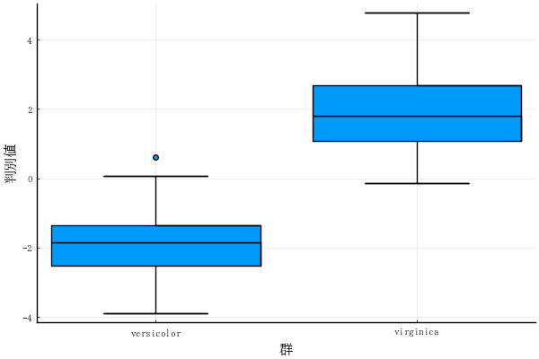
plotcandis(obj2, which="boxplot") # savefig("fig3.png")