#==========
Julia の修行をするときに,いろいろなプログラムを書き換えるのは有効な方法だ。
以下のプログラムを Julia に翻訳してみる。
正規確率紙に累積相対度数をプロットする
http://aoki2.si.gunma-u.ac.jp/R/npp2.html
npp2 <- function(x) # データベクトル
{
x <- x[!is.na(x)] # 欠損値を持つケースを除く
n <- length(x) # データの個数
x <- sort(x) # 昇順に並べ替える
y <- (1:n-0.5)/n # 累積相対度数
probs <- c(0.01, 0.1, 1, 5, 10, 20, 30, 40, 50, 60, 70, 80, 90, 95, 99, 99.9, 99.99)/100
plot(c(x[1], x[n]), qnorm(c(probs[1], probs[17])), type="n", yaxt="n",
xlab="Observed Value", ylab="Cumulative Percent",
main="Normal Probability Paper")
points(x, qnorm(y))
axis(2, qnorm(probs), probs*100)
}
ファイル名: npp2.jl 関数名:npp2
翻訳するときに書いたメモ
npp() よりは簡単?
指数乱数は randexp() だった。R はその他の分布型の乱数も用意されているのになあ。
==========#
using Distributions, Plots, Plots.PlotMeasures
function npp2(x; leftmargin=2mm, xlab = "観察値", ylab = "累積確率",
main = "正規確率紙")
pyplot()
x = collect(skipmissing(x))
n = length(x)
sort!(x)
y = (collect(1:n) .- 0.5) ./ n;
qny = quantile(Normal(), y);
probability = [0.01, 0.1, 1, 5, 10, 20, 30, 40, 50,
60, 70, 80, 90, 95, 99, 99.9, 99.99]/100;
qnp = quantile(Normal(), probability)
scatter(x, qny,
tickdirection=:out,
grid=false,
label="",
xlabel=xlab,
ylabel=ylab,
title=main,
leftmargin=leftmargin,
ylims=(minimum(qny), maximum(qny)),
size=(600, 400))
yticks!(qnp, string.(round.(probability, digits=4)))
hline!(qnp, linecolor = :gray, linestyle=:dot, label="")
end
using Random
Random.seed!(123)
x = randn(100) # 正規乱数
npp2(x)

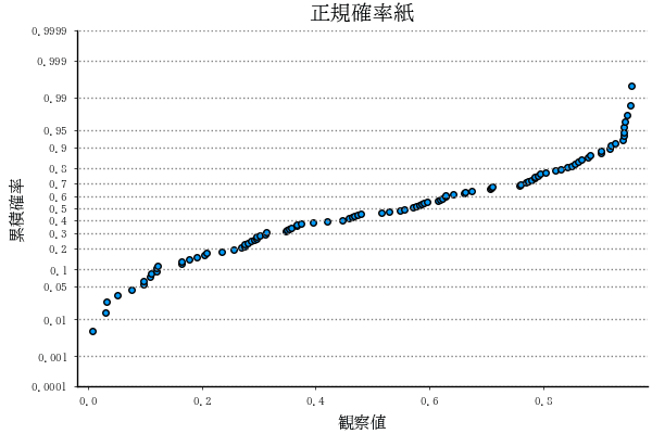
Random.seed!(123)
npp2(rand(100)) # 一様乱数
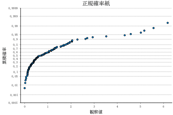
Random.seed!(123)
npp2(randexp(100)) # 指数乱数